Application: Dynamic analysis in human limb cell development
In this notebook, we will use the ModelComparison module from regvelo to evaluate different model training strategies. Using the best-performing model, we further demonstrate an in-silico perturbation analysis. The dataset used here is a subset of the human embryonic limb data from Zhang, B. et al, 2024, in which the authors profiled single-cell gene expression across post-conception weeks (PCW) 5 to 9. For our analysis, we focus specifically on cells from the lower limb that are involved in myogenic differentiation.
Using the selected model, we simulate transcription factor (TF) perturbations by removing all regulatory influences of the targeted TFs and generating the corresponding perturbed velocity fields. To quantify the impact of these perturbations, we compute the depletion likelihood as defined in Wang, W. et al, 2024. Additionally, we assess short-term perturbation effects by performing stochastic simulations of cell transitions under both the unperturbed and perturbed velocity fields.
Library import
# Basic packages
import numpy as np
import pandas as pd
import scipy
import torch
import matplotlib.pyplot as plt
import mplscience
import seaborn as sns
from scipy.stats import ttest_ind

# RegVelo and related package
import scanpy as sc
import cellrank as cr
import scvi
import scvelo as scv
import regvelo as rgv
from regvelo import REGVELOVI
from regvelo import ModelComparison # Import ModelComparison
General settings and helper functions
scvi.settings.seed = 0
scv.settings.verbosity = 3
cr.settings.verbosity = 2
%matplotlib inline
plt.rcParams["svg.fonttype"] = "none"
scv.settings.set_figure_params("scvelo", dpi=80, transparent=True, fontsize=14, color_map="viridis")
from typing import Dict, List, Tuple
import anndata
from matplotlib.axis import Axis

def add_significance(
    ax: Axis, left: int, right: int, significance: str, level: int = 0, orientation: str = "horizontal", **kwargs
) -> None:
    """Add significance bracket to Matplotlib Axis plot.

    Parameters
    ----------
    ax
        Matplotlib axis.
    left
        Position of left (top) subplot.
    right
        Position of right (bottom) subplot.
    siginifcance
        Significance ID to plot.
    level
        Level of bracket.
    orientation
        Orientation of bracket.
    **kwargs
        Keyword arguments passed to Axis.plot and to specify bracket level (`bracket_level`) and height
        (`bracket_height`), and distance between text and bracket (`text_height`).

    Returns
    -------
    None.
    """
    bracket_level = kwargs.pop("bracket_level", 1)
    bracket_height = kwargs.pop("bracket_height", 0.02)
    text_height = kwargs.pop("text_height", 0.01)

    if orientation == "horizontal":
        bottom, top = ax.get_ylim()
    else:
        bottom, top = ax.get_xlim()
    axis_range = top - bottom

    bracket_level = (axis_range * 0.07 * level) + top * bracket_level
    bracket_height = bracket_level - (axis_range * bracket_height)

    if orientation == "horizontal":
        ax.plot([left, left, right, right], [bracket_height, bracket_level, bracket_level, bracket_height], **kwargs)
        ax.text(
            (left + right) * 0.5,
            bracket_level + (axis_range * text_height),
            significance,
            ha="center",
            va="bottom",
            c="k",
        )
    else:
        ax.plot([bracket_height, bracket_level, bracket_level, bracket_height], [left, left, right, right], **kwargs)
        ax.text(
            bracket_level + (axis_range * text_height),
            (left + right) * 0.5,
            significance,
            va="center",
            ha="left",
            c="k",
            rotation=-90,
        )
Load data
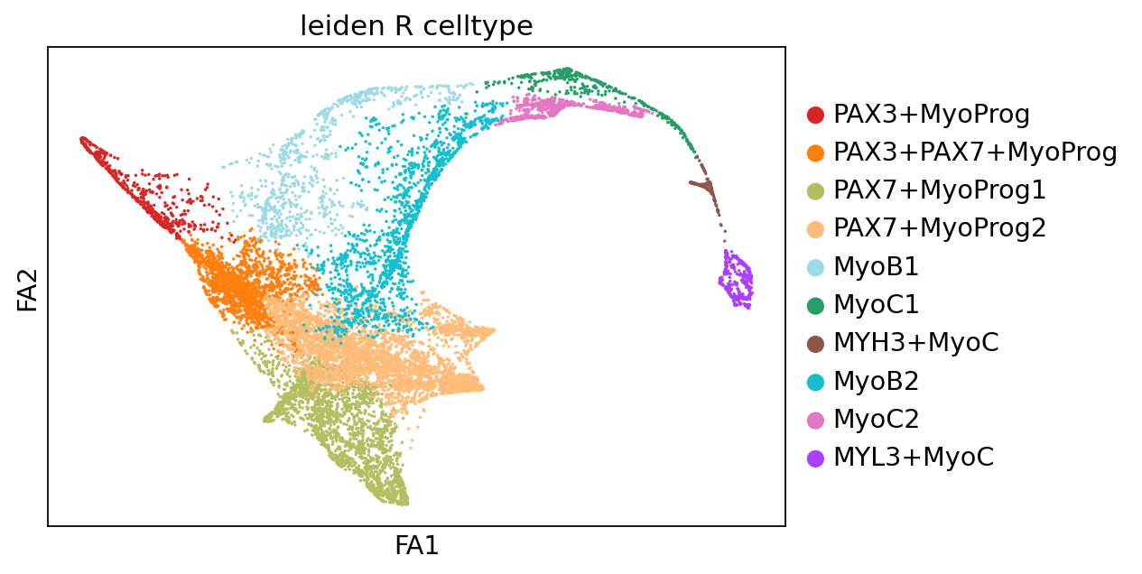
In this section, we load the limb development dataset described previously. The dataset contains 12207 cells and 606 genes. Celltype annotation are available in .obs['leiden_R_celltype'], including PAX7+MyoProg1, PAX7+MyoProg2, MyoB2, PAX3+PAX7+MyoProg, MyoC2, PAX3+MyoProg, MyoC1, MyoB1, MYL3+MyoC, and MYH3+MyoC cells.
The list of transcription factors (TFs) is stored in .var['TF'].
To evaluate model performance, we use the developmental stage number as ground truth for assessing the inferred latent time. This reference is later set via the argument side_information='Real_Time'.
adata = rgv.datasets.human_limb()
adata
AnnData object with n_obs × n_vars = 12207 × 606
    obs: 'percent_mito', 'n_counts', 'n_genes', 'doublet_scores', 'bh_pval', 'adj_stage', 'adj_sample', 'leiden', 'S_score', 'G2M_score', 'phase', 'leiden_R', 'leiden_R_celltype', 'initial_size_unspliced', 'initial_size_spliced', 'initial_size'
    var: 'Accession', 'Chromosome', 'End', 'Start', 'Strand', 'gene_ids', 'highly_variable', 'means', 'dispersions', 'dispersions_norm', 'velocity_genes', 'TF'
    uns: 'adj_stage_colors', 'celltype_sizes', 'diffmap_evals', 'draw_graph', 'leiden', 'leiden_R_celltype_colors', 'leiden_R_colors', 'leiden_sizes', 'log1p', 'marker_m_leiden_R_celltype', 'neighbors', 'network', 'paga', 'pca', 'phase_colors', 'rank_genes_groups', 'regulators', 'skeleton', 'targets', 'umap'
    obsm: 'X_diffmap', 'X_draw_graph_fa', 'X_pca', 'X_umap'
    layers: 'Ms', 'Mu', 'ambiguous', 'matrix', 'spliced', 'unspliced'
    obsp: 'connectivities', 'distances'
sc.pl.scatter(adata, basis="draw_graph_fa", color="leiden_R_celltype")
# infer Real_Time key
adata.obs['adj_stage_num'] = adata.obs['adj_stage'].str.replace('Pcw', '').astype(float)
adata.uns['skeleton'] = adata.uns['skeleton'].astype(np.float32)
adata
AnnData object with n_obs × n_vars = 12207 × 606
    obs: 'percent_mito', 'n_counts', 'n_genes', 'doublet_scores', 'bh_pval', 'adj_stage', 'adj_sample', 'leiden', 'S_score', 'G2M_score', 'phase', 'leiden_R', 'leiden_R_celltype', 'initial_size_unspliced', 'initial_size_spliced', 'initial_size', 'adj_stage_num'
    var: 'Accession', 'Chromosome', 'End', 'Start', 'Strand', 'gene_ids', 'highly_variable', 'means', 'dispersions', 'dispersions_norm', 'velocity_genes', 'TF'
    uns: 'adj_stage_colors', 'celltype_sizes', 'diffmap_evals', 'draw_graph', 'leiden', 'leiden_R_celltype_colors', 'leiden_R_colors', 'leiden_sizes', 'log1p', 'marker_m_leiden_R_celltype', 'neighbors', 'network', 'paga', 'pca', 'phase_colors', 'rank_genes_groups', 'regulators', 'skeleton', 'targets', 'umap'
    obsm: 'X_diffmap', 'X_draw_graph_fa', 'X_pca', 'X_umap'
    layers: 'Ms', 'Mu', 'ambiguous', 'matrix', 'spliced', 'unspliced'
    obsp: 'connectivities', 'distances'
Model Comparison
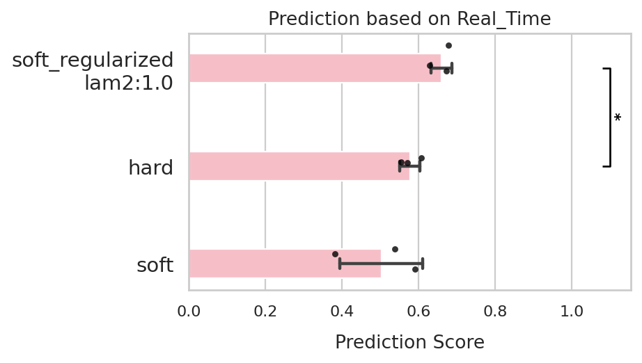
In the following section, we compare different model training strategies, i.e. soft, hard, and soft_regularized modes under the same normalization factor. Model performance is evaluated using real developmental time as side information (side_information = 'Real_time').
We first define the set of terminal states, which includes PAX7+MyoProg1, MYH3+MyoC, and MYL3+MyoC cells. Additionally, we set n_states=8.
TERMINAL_STATES = ["PAX7+MyoProg1", "MYH3+MyoC", "MYL3+MyoC"]
n_STATES = 8
comp = ModelComparison(terminal_states=TERMINAL_STATES, n_states=n_STATES)
comp.train(adata=adata,
           model_list=['soft','hard','soft_regularized'],
           lam2=[1.0],
           n_repeat=3)
Monitored metric elbo_validation did not improve in the last 45 records. Best score: -1754.909. Signaling Trainer to stop.
Monitored metric elbo_validation did not improve in the last 45 records. Best score: -1718.788. Signaling Trainer to stop.
Monitored metric elbo_validation did not improve in the last 45 records. Best score: -1734.265. Signaling Trainer to stop.
Monitored metric elbo_validation did not improve in the last 45 records. Best score: -1524.247. Signaling Trainer to stop.
Monitored metric elbo_validation did not improve in the last 45 records. Best score: -1505.458. Signaling Trainer to stop.
Monitored metric elbo_validation did not improve in the last 45 records. Best score: -1310.308. Signaling Trainer to stop.
['soft_0',
 'soft_1',
 'soft_2',
 'hard_0',
 'hard_1',
 'hard_2',
 'soft_regularized\nlam2:1.0_0',
 'soft_regularized\nlam2:1.0_1',
 'soft_regularized\nlam2:1.0_2']
comp.evaluate(side_information='Real_Time',
              side_key='adj_stage_num')
comp.plot_results(side_information='Real_Time')
comp.df_Real_Time
| Model | Corr | Run | |
|---|---|---|---|
| 0 | soft | 0.537389 | 0 |
| 1 | soft | 0.590243 | 1 |
| 2 | soft | 0.381020 | 2 |
| 3 | hard | 0.570352 | 0 |
| 4 | hard | 0.554766 | 1 |
| 5 | hard | 0.606984 | 2 |
| 6 | soft_regularized\nlam2:1.0 | 0.629149 | 0 |
| 7 | soft_regularized\nlam2:1.0 | 0.678848 | 1 |
| 8 | soft_regularized\nlam2:1.0 | 0.672296 | 2 |
Based on the results, we can see that the best-performing model is the soft_regularized mode, which achieves the highest prediction score while maintaining good stability across runs. We therefore use this model to demonstrate the following perturbation analysis.
vae_sr0 = comp.MODEL_TRAINED['soft_regularized\nlam2:1.0_0']
vae_sr0.save('vae_sr0')
In silico perturbation
In the following analysis, we sequentially knock down two TFs, MSC and MYOG, to examine their effects on cell fate determination. Musculin (MSC) is identified as an important transcriptional repressor that maintains muscle stem cell identity, while MYOG gene promotes terminal differentiation Zhang, B. et al, 2024.
For each TF, we use RegVelo’s rgv.tl.in_silico_block_simulation function to remove its regulatory effects from the best-performing model and generate the corresponding perturbed velocity field.
# Reload selected model
vae_sr0 = REGVELOVI.load('vae_sr0', adata)
rgv.tl.set_output(adata, vae_sr0, n_samples=30, batch_size=adata.n_obs)
INFO File vae_sr0/model.pt already downloaded
# Computing states transition probability
vk = cr.kernels.VelocityKernel(adata).compute_transition_matrix()
ck = cr.kernels.ConnectivityKernel(adata).compute_transition_matrix()
estimator = cr.estimators.GPCCA(0.8*vk + 0.2*ck)
estimator.compute_macrostates(n_states=n_STATES, cluster_key='leiden_R_celltype')
estimator.set_terminal_states(TERMINAL_STATES)
estimator.compute_fate_probabilities()
Computing transition matrix using `'deterministic'` model
Using `softmax_scale=10.3188`
    Finish (0:00:32)
Computing transition matrix based on `adata.obsp['connectivities']`
    Finish (0:00:00)
Computing Schur decomposition
WARNING: Using `8` components would split a block of complex conjugate eigenvalues. Using `n_components=9`
When computing macrostates, choose a number of states NOT in `[8]`
Adding `adata.uns['eigendecomposition_fwd']`
       `.schur_vectors`
       `.schur_matrix`
       `.eigendecomposition`
    Finish (0:00:17)
WARNING: Unable to compute macrostates with `n_states=8` because it will split complex conjugate eigenvalues. Using `n_states=9`
Computing `9` macrostates
Adding `.macrostates`
       `.macrostates_memberships`
       `.coarse_T`
       `.coarse_initial_distribution
       `.coarse_stationary_distribution`
       `.schur_vectors`
       `.schur_matrix`
       `.eigendecomposition`
    Finish (0:00:06)
Adding `adata.obs['term_states_fwd']`
       `adata.obs['term_states_fwd_probs']`
       `.terminal_states`
       `.terminal_states_probabilities`
       `.terminal_states_memberships
    Finish`
Computing fate probabilities
Adding `adata.obsm['lineages_fwd']`
       `.fate_probabilities`
    Finish (0:00:00)
adata_pert_dict = {}
TF_list = ['MSC','MYOG']
MODEL = 'vae_sr0'
for TF in TF_list:
    adata_target_pert, reg_vae_pert = rgv.tl.in_silico_block_simulation(model=MODEL,
                                                                        adata=adata,
                                                                        TF=TF,
                                                                        cutoff=0)
    adata_pert_dict[TF] = adata_target_pert
INFO     File vae_sr0/model.pt already downloaded
INFO     File vae_sr0/model.pt already downloaded
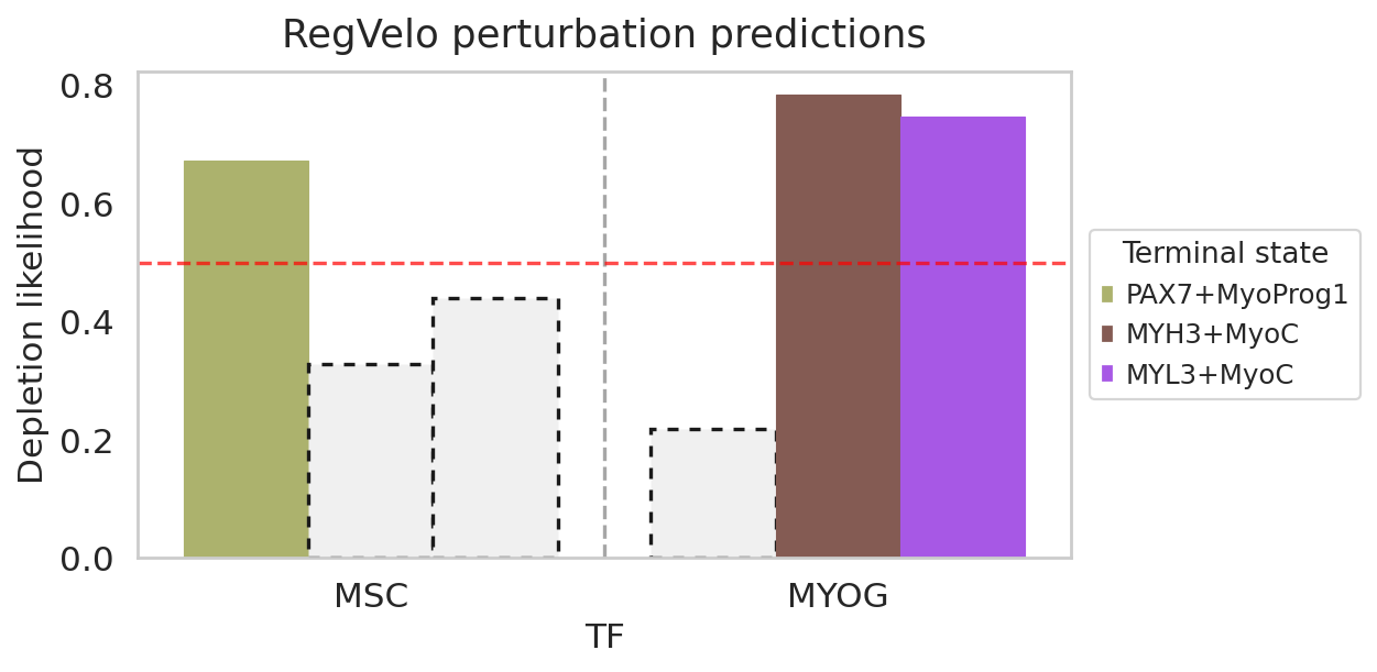
Long-term perturbation effect (Depletion likelihood based on cell fate probabilities)
We assess the perturbation effects on cell fate decisions by passing the perturbed velocity estimates into CellRank’s VelocityKernel. To quantify the impact on terminal cell states, we compute depletion scores using rgv.mt.depletion_score and visualize the results using rgv.pl.depletion_score.
ct_indices = {
    ct: adata.obs["term_states_fwd"][adata.obs["term_states_fwd"] == ct].index.tolist()
    for ct in TERMINAL_STATES}

# Computing states transition probability for perturbed systems
for TF, adata_target_perturb in adata_pert_dict.items():
    vk = cr.kernels.VelocityKernel(adata_target_perturb).compute_transition_matrix()
    ck = cr.kernels.ConnectivityKernel(adata_target_perturb).compute_transition_matrix()
    estimator = cr.estimators.GPCCA(0.8*vk + 0.2*ck)
    estimator.compute_macrostates(n_states=n_STATES, cluster_key='leiden_R_celltype')
    estimator.set_terminal_states(ct_indices)
    estimator.compute_fate_probabilities()

    adata_pert_dict[TF] = adata_target_perturb
Computing transition matrix using `'deterministic'` model
Using `softmax_scale=10.3111`
    Finish (0:00:06)
Computing transition matrix based on `adata.obsp['connectivities']`
    Finish (0:00:00)
Computing Schur decomposition
Adding `adata.uns['eigendecomposition_fwd']`
       `.schur_vectors`
       `.schur_matrix`
       `.eigendecomposition`
    Finish (0:00:00)
Computing `8` macrostates
Adding `.macrostates`
       `.macrostates_memberships`
       `.coarse_T`
       `.coarse_initial_distribution
       `.coarse_stationary_distribution`
       `.schur_vectors`
       `.schur_matrix`
       `.eigendecomposition`
    Finish (0:00:04)
Adding `adata.obs['term_states_fwd']`
       `adata.obs['term_states_fwd_probs']`
       `.terminal_states`
       `.terminal_states_probabilities`
       `.terminal_states_memberships
    Finish`
Computing fate probabilities
Adding `adata.obsm['lineages_fwd']`
       `.fate_probabilities`
    Finish (0:00:00)
Computing transition matrix using `'deterministic'` model
Using `softmax_scale=10.2384`
    Finish (0:00:06)
Computing transition matrix based on `adata.obsp['connectivities']`
    Finish (0:00:00)
Computing Schur decomposition
Adding `adata.uns['eigendecomposition_fwd']`
       `.schur_vectors`
       `.schur_matrix`
       `.eigendecomposition`
    Finish (0:00:00)
Computing `8` macrostates
Adding `.macrostates`
       `.macrostates_memberships`
       `.coarse_T`
       `.coarse_initial_distribution
       `.coarse_stationary_distribution`
       `.schur_vectors`
       `.schur_matrix`
       `.eigendecomposition`
    Finish (0:00:04)
Adding `adata.obs['term_states_fwd']`
       `adata.obs['term_states_fwd_probs']`
       `.terminal_states`
       `.terminal_states_probabilities`
       `.terminal_states_memberships
    Finish`
Computing fate probabilities
Adding `adata.obsm['lineages_fwd']`
       `.fate_probabilities`
    Finish (0:00:00)
df = rgv.mt.cellfate_perturbation(perturbed=adata_pert_dict, baseline=adata, terminal_state=TERMINAL_STATES)
df
| Depletion likelihood | p-value | FDR adjusted p-value | Terminal state | TF | |
|---|---|---|---|---|---|
| 0 | 0.671613 | 0.0 | 0.0 | PAX7+MyoProg1 | MSC |
| 1 | 0.327251 | 1.0 | 1.0 | MYH3+MyoC | MSC |
| 2 | 0.439194 | 1.0 | 1.0 | MYL3+MyoC | MSC |
| 0 | 0.218008 | 1.0 | 1.0 | PAX7+MyoProg1 | MYOG |
| 1 | 0.784527 | 0.0 | 0.0 | MYH3+MyoC | MYOG |
| 2 | 0.747119 | 0.0 | 0.0 | MYL3+MyoC | MYOG |
rgv.pl.cellfate_perturbation(adata=adata,
                             df=df,
                             fontsize=14,
                             figsize=(8,4),
                             legend_loc='center left',
                             legend_bbox=(1.02, 0.5),
                             color_label="leiden_R_celltype")
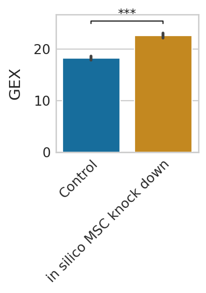
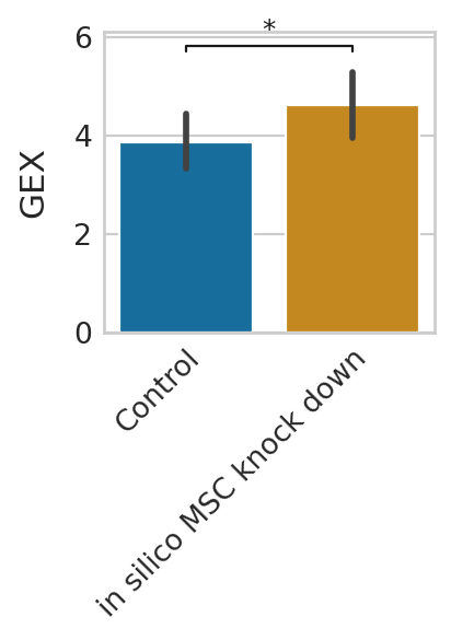
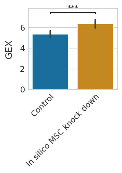
Gene expression prediction under pertubation
We can further predict gene expression levels using rgv_expression_fit and compare the results to the control data. We demonstrate this using three representative genes and visualize the in-silico perturbation effects on their expression level.
Ms, Mu = vae_sr0.rgv_expression_fit(return_numpy=True, n_samples=30)
adata.layers["fit_s"] = Ms
adata.layers["fit_u"] = Mu
adata_perturb, vae_perturb = rgv.tl.in_silico_block_simulation(MODEL, adata, "MSC", effects=0)
adata_perturb.layers["fit_s"],adata_perturb.layers["fit_u"] = vae_perturb.rgv_expression_fit(n_samples=30)
INFO File vae_sr0/model.pt already downloaded
genes = ["MYOG", "MYH3", "TNNT1"]

for g in genes:
    df = pd.DataFrame(
        {
            "GEX": adata[:,g].layers["fit_s"].flatten().tolist() + adata_perturb[:,g].layers["fit_s"].flatten().tolist(),
            "Condition": ["Control"] * adata.shape[0] + ["in silico MSC knock down"] * adata.shape[0],
        }
    )
    df["GEX"] = df["GEX"] * np.max(adata[:,g].layers["spliced"])

    with mplscience.style_context():
        sns.set_style(style="whitegrid")
        fig, ax = plt.subplots(figsize=(3, 4))

        sns.barplot(data=df, x="Condition", y="GEX", palette="colorblind", ax=ax)

        ax.set_ylabel("GEX", labelpad=10)
        ax.set_xlabel("")
        ax.set_xticklabels(ax.get_xticklabels(), rotation = 45, ha = 'right', rotation_mode = 'anchor')
        plt.tight_layout(pad=2)
        ttest_res = ttest_ind(
            adata_perturb[:,g].layers["fit_s"].flatten().tolist(),
            adata[:,g].layers["fit_s"].flatten().tolist(),
            alternative="greater"
        )
        significance = rgv.mt.get_significance(ttest_res.pvalue)
        add_significance(
            ax=ax,
            left=0,
            right=1,
            significance=significance,
            lw=1,
            bracket_level=1.05,
            c="k",
            level=0,
        )

        plt.show()
Short-term perturbation effect (Stochastic simulations of cell transitions)
To assess short-term perturbation effects, we compare the dynamics of the perturbed and unperturbed models using stochastic simulations of cell transitions. Transition matrices are computed using CellRank based on the original and perturbed velocity fields.
For the initial state, we select cells annotated as PAX3+MyoProg and define the start_indices and terminal_indices, which are required for the rgv.tl.markov_density_simulation function. This function simulates trajectories across a velocity-based Markov chain and returns the absolute and relative number of visits to each terminal state, stored in .obs['visits'] and .obs['visits_dens'], respectively.
To quantify the effect of perturbation, we apply rgv.tl.simulated_density_diff, which computes the average difference in visit counts between the perturbed and control systems for each terminal state. Negative values indicate a depletion of visits in the perturbed system relative to the control. The function also performs a paired t-test (scipy.stats.ttest_rel) to determine whether these differences are statistically significant. The resulting p-values are returned alongside the mean differences.
start_indices = np.where(adata.obs["leiden_R_celltype"].isin(["PAX3+MyoProg"]))[0]
terminal_indices = np.where(adata.obs["term_states_fwd"].isin(TERMINAL_STATES))[0]

vk = cr.kernels.VelocityKernel(adata).compute_transition_matrix()
ck = cr.kernels.ConnectivityKernel(adata).compute_transition_matrix()
combined_kernel = 0.8*vk + 0.2*ck
combined_kernel_t = combined_kernel.transition_matrix.A
Computing transition matrix using `'deterministic'` model
Using `softmax_scale=10.3188`
    Finish (0:00:06)
Computing transition matrix based on `adata.obsp['connectivities']`
    Finish (0:00:00)
method = "stepwise"

TF = "MSC"
adata_perturb = adata_pert_dict[TF]

vk_p = cr.kernels.VelocityKernel(adata_perturb).compute_transition_matrix()
ck_p = cr.kernels.ConnectivityKernel(adata_perturb).compute_transition_matrix()
combined_kernel_p = 0.8*vk_p + 0.2*ck_p
combined_kernel_pt = combined_kernel_p.transition_matrix.A
Computing transition matrix using `'deterministic'` model
Using `softmax_scale=10.3111`
    Finish (0:00:06)
Computing transition matrix based on `adata.obsp['connectivities']`
    Finish (0:00:00)
total_simulations = rgv.tl.markov_density_simulation(adata,
                                                     combined_kernel_t,
                                                     start_indices,
                                                     terminal_indices,
                                                     TERMINAL_STATES,
                                                     method=method)
_ = rgv.tl.markov_density_simulation(adata_perturb,
                                     combined_kernel_pt,
                                     start_indices,
                                     terminal_indices,
                                     TERMINAL_STATES,
                                     method=method)
dd_score, dd_sig = rgv.tl.simulated_visit_diff(adata, adata_perturb, TERMINAL_STATES)
print(dd_score)
print(dd_sig)
[-137.39999999999998, 2990.7333333333345, 0.5666666666666664]
[8.709956977564526e-05, 0.00047703174620153616, 0.6583323305783767]
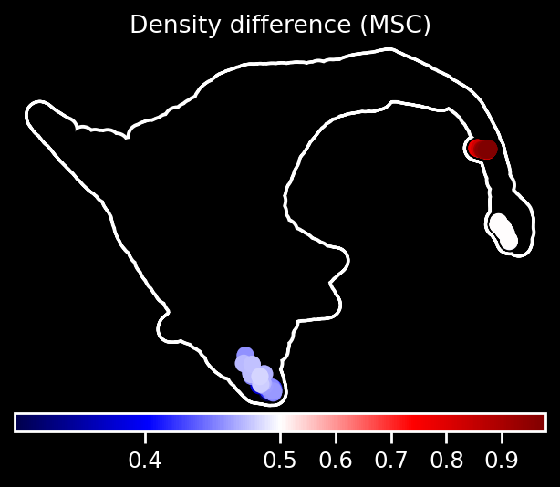
We further use the function rgv.pl.simulated_density_diff to visualize short-term perturbation effects by analyzing the number of simulated visits to each terminal cell in both the perturbed and unperturbed systems. For each terminal cell, we compute the difference in the number of visits between the perturbed and control simulations. To account for stochastic variability across simulations, this difference is scaled by \(1/\sqrt{\text{\# total simulations}}\). The resulting scaled differences are then passed through a sigmoid function and stored in adata.obs['visits_diff']. These scores are then smoothed over neighboring cells to produce a spatially coherent signal, stored in adata.obs['visits_diff_smoothed']. Values below 0.5 indicate a relative depletion of visits to the corresponding terminal cell under perturbation.
rgv.pl.simulated_visit_diff(adata,
                            adata_perturb,
                            TERMINAL_STATES,
                            total_simulations,
                            basis="draw_graph_fa",
                            color_map="seismic",
                            title="Density difference (MSC)")